Introduction to Micro Economics
3. Monopoly and Market Power
3.2. Monopoly Characteristics
Monopoly Characteristics
3.4.1 The Absence of a Supply Curve for a Monopolist
There is no supply curve for a monopolist. This differs from a competitive industry, where there is a one-to-one correspondence between price (P) and quantity supplied (Qs). For a monopoly, the price depends on the shape of the demand curve, as shown in Figure 3.11. A mathematical “function” is defined as a one-to-one correspondence between each point in the range (x) and the domain . A supply curve, then, requires a single price (P) for each quantity (Q). This graph shows that there is more than one price associated with each quantity. At quantity Q0, for demand curve D1, the monopolist maximizes profits by setting MR1 = MC, which results in price P1. However, for demand curve D2, the monopolist would set MR2=MC, and charge a lower price, P2. Since there is more than one price associated with a single quantity (Q0), there is no one-to-one correspondence between price and quantity supplied, and no supply curve for a monopolist.
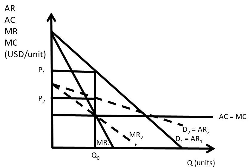
Figure 3.11 Absence of a Supply Curve for a Monopolist
3.4.2 The Effect of a Tax on a Monopolist’s Price
In a competitive industry, a tax results in an increase in price that is based on the incidence of the tax. The price increase is a fraction of the tax, less than the tax amount. The tax incidence depends on the magnitude of the elasticities of supply and demand. In a monopoly, it is possible that the price increase from a tax is greater than the tax itself, as shown in Figure 3.12. This is an interesting and nonintuitive result!
Before the tax, the monopolist sets MR = MC at Q0, and sets price at P0. After the tax is imposed, the marginal costs increase to C + t. The monopolist sets MR = MC = C + t, produces quantity Q1, and charges price P1. The increase in price (P1 – P0) is larger than the tax rate (t), the vertical distance between the C + t and MC lines. In this case, consumers of the monopoly good are paying more than 100 percent of the tax rate. This is because of the shape of the demand curve: it is profitable for the monopoly to reduce quantity produced to increase the price.
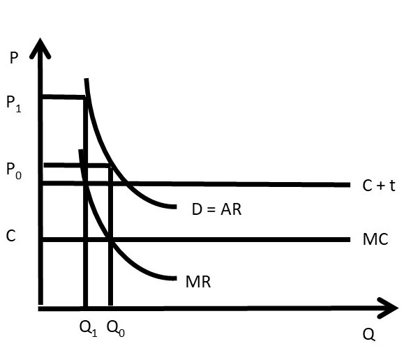
Figure 3.12 The Effect of a Tax on a Monopolist’s Price
3.4.3 Multiplant Monopolist
Suppose that a monopoly has two or more plants (factories). How does the monopolist determine how much output should be produced at each plant? Profit-maximization suggests two guidelines for the multiplant monopolist. Suppose that the monopolist operates n plants.
(1) Set MC equal across all plants: MC1 = MC2 = … =MCn, and
(2) Set MR = MC in all plants.
A mathematical model of a multiplant monopolist demonstrates profit-maximization. The result is interesting and important, as it shows that multiplant firms will not always close older, less efficient plants. This is true even if the older plants have higher production costs than newer, more efficient plants.
Suppose that a monopolist has two plants, and total output (QT) is the sum of output produced in plant 1 (Q1) and plant 2 (Q2).
(3.6) Q1 + Q2 = QT
The profit-maximizing model for the two-plant monopolist yields the solution. The costs of producing output in each plant differ. Assume that the old plant (plant 1) is less efficient than the new plant (plant 2): C1 > C2.
max π = TR – TC
= P(QT)QT – C1(Q1) – C2(Q2)
∂π/∂Q1 = ∂TR/∂Q1 – C1’(Q1) = 0
∂π/∂Q2 = ∂TR/∂Q2 – C2’(Q2) = 0
The profit-maximizing solution is:
(3.7) MR = MC1 = MC2
The multiplant monopolist solution is shown in Figure 3.13. The marginal cost curve for plant 1 is higher than the marginal cost curve for plant 2, reflecting the older, less efficient plant. Rather than shutting the less efficient plant down, the monopolist should produce some output in each plant, and set the MC of each plant equal to MR, as shown in the graph. Let MCT be the total (sum) of the marginal cost curves: MT = MC1 + MC2. The profit maximizing quantity (QT) is found by setting MR equal to MCT. At the profit maximizing quantity (QT), the monopolist sets price equal to P, found by plugging QT into the consumers’ willingness to pay, or the demand curve (D).
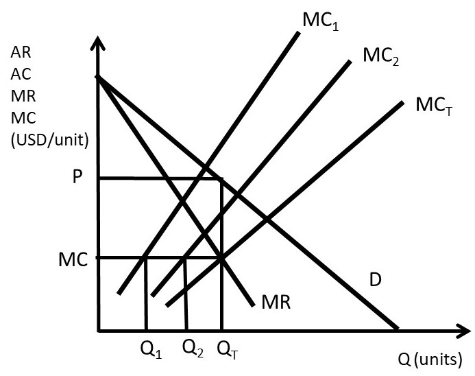
Figure 3.13 Multiplant Monopolist
To find the quantity to produce in each plant, the firm sets MC1 = MC2 = MCT to find the profit-maximizing level of output in each plant: Q1 and Q2. The outcome of the multiplant monopolist yields useful conclusions for any firm: continue using any input, plant, or resource until marginal costs equal marginal revenues. Less efficient resources can be usefully employed, even if more efficient resources are available. The next section will explore the determinants and measurement of monopoly power, also called market power.
3.5 Monopoly Power
In this section, the determinants and measurement of monopoly power are examined.
3.5.1 The Lerner Index of Monopoly Power
Economists use the Lerner Index to measure monopoly power, also called market power. The index is the percent markup of price over marginal cost.
(3.8) L = (P – MC)/P
The Lerner Index is a positive number (L ≥ 0), increasing in the amount of market power. A perfectly competitive firm has a Lerner Index equal to zero (L = 0), since price is equal to marginal cost (P = MC). A monopolist will have a Lerner Index greater than zero, and the index will be determined by the amount of market power that the firm has. A larger Lerner Index indicates more market power. In Section 3.3.3, a Pricing Rule was derived: (P – MC)/P = – 1/Ed, where Ed is the price elasticity of demand. Substitution of this pricing rule into the definition of the Lerner Index provides the relationship between the percent markup and the price elasticity of demand.
(3.9) L = (P – MC)/P = – 1/Ed
An example of a Lerner Index might be Big Macs. There are substitutes available for Big Macs, so if the price increases, consumers can buy a competing brand such as Whoppers. In the case of a good with close substitutes, the price elasticity of demand is larger (more elastic), causing the percent markup to be smaller: the Lerner Index is relatively small. A monopoly is defined as a single seller in an industry with no close substitutes. Therefore, a monopoly that produces a good with no close substitutes would have a higher Lerner Index.
A second pricing rule can be derived from equation (3.9), if we assume that the firm maximizes profits (MR = MC). In that case, the relationship between price and marginal revenue is equal to: MR = P(1 + 1/Ed). If profit-maximization (MR = MC) is assumed, then:
(3.10) MC = P(1 + 1/Ed)
Rearranging:
(3.11) P = MC/(1 + 1/Ed)
This is a useful equation, as it relates price to marginal cost. For example, a perfectly competitive firm has a perfectly elastic demand curve (Ed = negative infinity). Substitution of this elasticity into the pricing rule yields P = MC. For a monopoly that has a price elasticity equal to –2, P = 2MC. The price is two times the production costs in this case. To summarize:
(1) if Ed is large, the firm has less market power, and a small markup
(2) if Ed is small, the firm has more market power, and a large markup.
A monopoly example is useful to review monopoly and the Lerner Index. Suppose that the inverse demand curve facing a monopoly is given by: P = 500 – 10Q. The monopoly production costs are given by: C(Q) = 10Q2 + 100Q. Profit-maximization yields the optimal monopoly price and quantity.
max π = TR – TC
= P(Q)Q – C(Q)
= (500 – 10Q)Q – (10Q2 + 100Q)
= 500Q – 10Q2 – 10Q2 – 100Q
∂π/∂Q= 500 – 20Q – 20Q – 100 = 0
40Q = 400
Q* = 10 units
P* = 500 – 10Q* = 500 – 100 = 400 USD/unit.
To calculate the value of the Lerner Index, price and marginal cost are needed (equation 3.9).
MC = C’(Q) = 20Q + 100.
MC* = 20(10) + 100 = 300 units
L = (P – MC)/P = (400 – 300)/400 = 100/400 = 0.25
This result can be checked with the pricing rule: (P – MC)/P = – 1/Ed.
Ed = (∂Q/∂P)(P/Q)
For this monopoly, ∂P/∂Q = –10. This is the first derivative of the inverse demand function. Therefore, ∂Q/∂P = – 1/10.
Ed = (∂Q/∂P)(P/Q) = (– 1/10)(400/10) = – 400/100 = – 4.
L = (P – MC)/P = – 1/Ed = –1/–4 = 0.25.
The same result was achieved using both methods, so the Lerner Index for this monopoly is equal to 0.25.
3.5.2 Welfare Effects of Monopoly
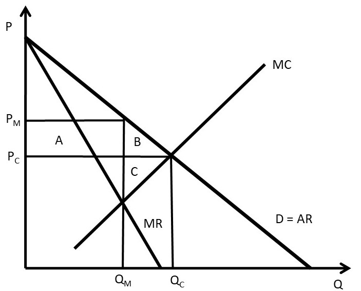
The welfare effects of a market or policy change are summarized as, “who is helped, who is hurt, and by how much.” To measure the welfare impact of monopoly, the monopoly outcome is compared with perfect competition. In competition, the price is equal to marginal cost (P = MC), as in Figure 3.14. The competitive price and quantity are Pc and Qc. The monopoly price and quantity are found where marginal revenue equals marginal cost (MR = MC): PM and QM. The graph indicates that the monopoly reduces output from the competitive level in order to increase the price (PM > Pc and QM < Qc). The welfare analysis of a monopoly relative to competition is straightforward.
ΔCS = – AB
ΔPS = +A – C
ΔSW = – BC
DWL = BC
Consumers are losers, and the benefits of monopoly depend on the magnitudes of areas A and C. Since a monopolist faces an inelastic supply curve (no close substitutes), area A is likely to be larger than area C, making the net benefits of monopoly positive.